Rearranging Data with New Functions in Excel

Rearranging Data with New Functions

In this article, we’ll explore these new functions: TOCOL, TOROW, WRAPCOLS, WRAPROWS, CHOOSECOLS, CHOOSEROWS

Let’s start with TOCOL. This function takes an array of values and stacks them into one column. Suppose, for example, we have this data:

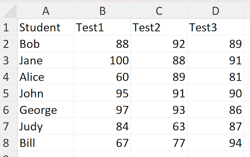
And we just want to list the scores vertically. The TOCOL function is designed just for this purpose. Its syntax is =TOCOL(array, ignore, scan_by_column). The array above is B2:D8. “Ignore” means to skip over any blank cells. “Scan_by_column” will be examined in a moment.

Here’s the result:

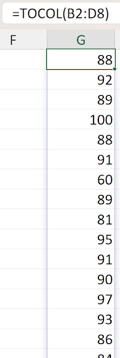
Notice the values are picked from Bob’s test scores, row 2, columns B, then C, then D, before it wraps to row 3. If you wanted to make it go down then over (rather than over then down), that’s where the last parameter comes into play:

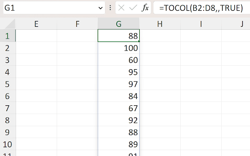
You can see that these values are from Test1, before it moves on to Test2 in cell G8.

The function TOROW works the same way as TOCOL, but horizontally. The same data as the last example is here:

This is also the same as =TRANSPOSE(TOCOL(B2:B8,, TRUE)), but that’s a bit of overkill, since we do have the TOROW function!

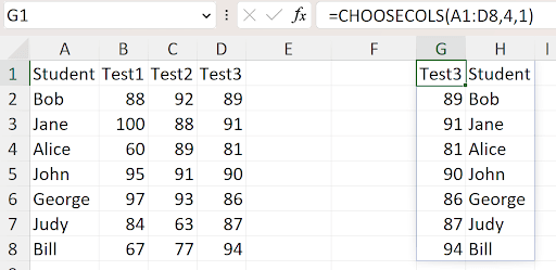
Let’s take a look at the CHOOSECOLS function. Without it, you get all the columns you’ve referenced, but with it, you can select which ones you want to see. For example, let’s say you wanted to just show the names and Test3 scores from the original data.

This does the trick:

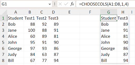
The CHOOSECOLS was given the array (A1:D8), then the list of columns to be shown – the 1st and 4th. You can also rearrange them:

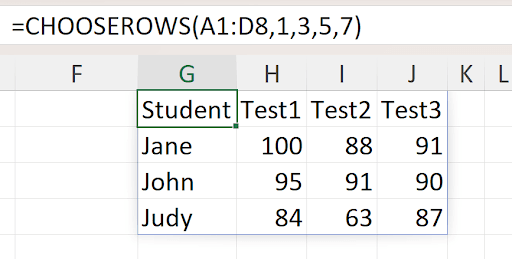
CHOOSEROWS works similarly. If we only wanted to see the4 students which begin with J (and the header):

Suppose you wanted to see a vertical list of the above results, including the names:

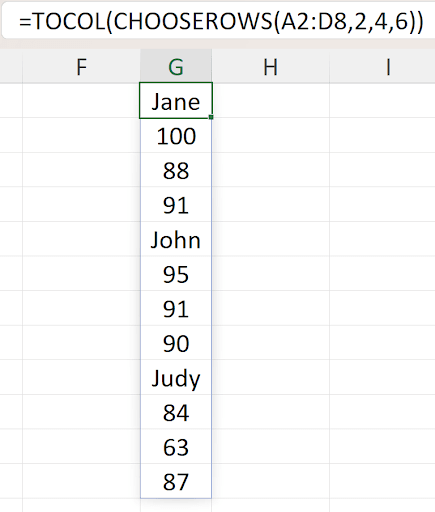
First, the range referenced was A2:D8 (no headers), then the J-students were selected by the 2,4,6 in the CHOOSEROWS function. Passing that to the TOCOL function did the trick!

Let’s examine WRAPROWS and WRAPCOLS. These are sort of the opposite of TOROW and TOCOL! Here’s the data we’ll look at to begin with:

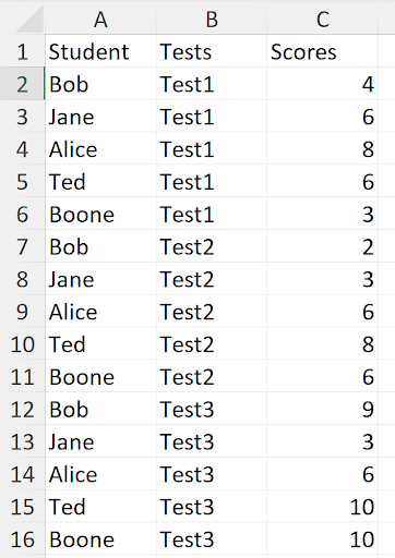
We want to reorganize it to look like this:

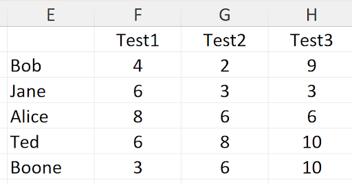
This was done with 3 functions! They were entered in cells F1, E2, and F2.

Let’s first look at the function in F1:

This wraps the UNIQUE function inside the TOROW function. Otherwise, the UNIQUE function entered in F1 would return the values all in column F. This could have been =TRANSPOSE(UNIQUE(B2:B16)) but you should start getting comfortable with the new functions to have more tools in your toolbox!

The formula in E2 is:

Simple enough. Okay, what’s in F2? It’s the WRAPCOLS function.

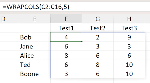
The array being referenced is the vertical list of scores. The “5” in the function says that after 5 rows, wrap the result into the next column. Test1 has 5 scores to it (as do the others), so after the 3 is reached in cell F6, it wraps to the next column.

Now suppose the original data was sorted differently:

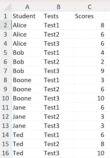
The order is Student, then tests. So, the data is “grouped” into 3 rows. To get the similar results as above, we now need the WRAPROWS function in cell F2:

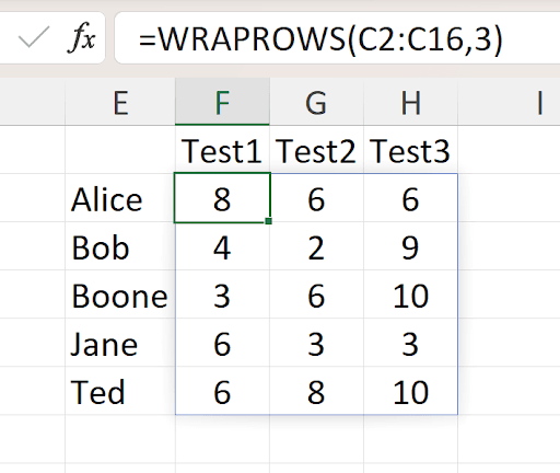
Notice that after every 3 columns, we want to wrap to the next row.