How to Add Headers & Footers in Excel: More Fun with Excel's Page Layout Tab

In this blog, we’ll complete the discussion of what’s available on the Page Layout tab and a few other items. The Header/Footer tab of the Page Setup dialog is where we left off. Let’s look at this again. Click the dialog launcher below the Print Titles icon and then click the 3^rd tab (Header/Footer), and you see: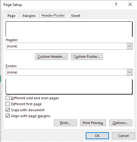

The main buttons here are the Custom Header and Custom Footer buttons. Either gives the identical dialog aside from the results being shown in the Header or the Footer. The dialog looks like this:

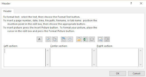
Before we go into all these buttons, notice the tab, “Header” at the top of the dialog. If, in the previous dialog, the box “Different odd and even pages” was checked, then when the Custom Header button is clicked you’d see these tabs at the top:

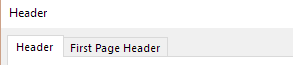
And if the “Different first page” was checked, then you’d see these tabs at the top:

And if both were checked, you’d see these tabs:

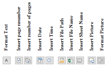
The icons in the middle of the dialog are these:

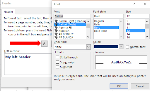
If you type “My left header” in the left section, then select that text, then click the Format Text icon (pointed to by the arrow), you will get the Font dialog as shown, where you can format the selected text. What’s shown here is the effect of doing exactly that, then issuing the command again where you can see the result of the text’s formatting:

In the next dialog, the cursor was placed in the Center section, the page number icon was selected, then the word “of” was typed (surrounded by a space), then the number of pages icon was selected:

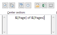
The &[Page] and &[Pages] are “codes” for Excel to insert the current page and total number of pages. For example, the following preview would show if this were done to the center section of the footer on a document with 19 pages and we were looking at page 2:

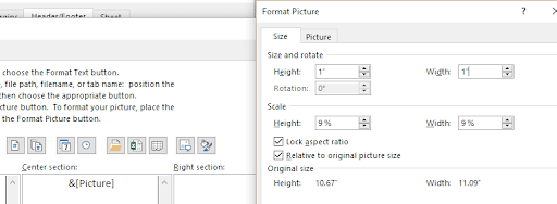
Some of the other commands are pretty self-explanatory. Here, the Insert Picture icon was selected (an Excel logo was chosen), then the Format picture icon was chosen where the image was set to be 1” X 1”:

---

The result:

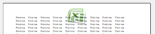
If the margins are also set, then this could show as:

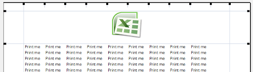
Where can you set the margins in the Print preview? Scroll down a bit and you’ll see 2 icons at the bottom right, quite hidden from the user (!) – Notice the red arrow:

The left button is the toggle for the margins, which you can then drag around, and the right one is to zoom in to the page.

The last icons on the Page Layout tab we’re discussing are these:

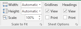
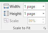
The # of pages wide or tall can be set, or the scale can be set. For example, if you set both Width and Height to 1 page, then the Scale would automatically be set (and no longer enabled), something like this:

The last 4 checkboxes are used to display and/or print the gridlines or headings (headings being the row numbers and column letters).

Suppose you make all your page settings as you like, and then realize you have other sheets to which you’d like to make the same settings. Do you have to repeat all the steps for each sheet? No! You can CTRL/click or shift/click the other worksheet tabs to put them into a group. Here, Sheet4 is active, but Sheet3 is now part of the group:

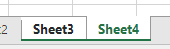
The top of the screen shows this:

---

The word [group] indicates more than one sheet is included in the group.

Now all you need do is bring up the page setup dialog and simply click OK! The settings for the active sheet are copied to all the other sheets in the group!

If you click on the Page Break Preview icon at the bottom right of the screen,

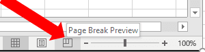  you would see an editable preview of the printout:

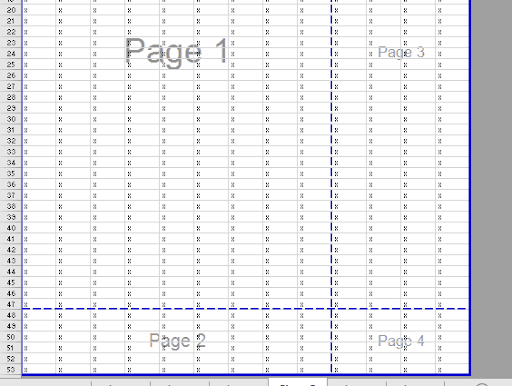
The dotted lines indicate where the page breaks will automatically occur. You can actually click and drag these to a new location. If you drag the vertical break to the right, you would be inserting a manual page break. Here’s the same data with the vertical break dragged all the way to the right and the horizontal line dragged to the bottom:

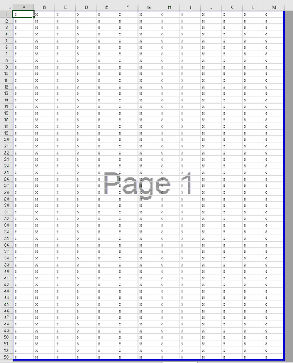
The icon to the left of the Page Break preview at the bottom of the Excel screen is the Page Layout tab. This gives the following view:

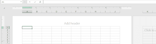
Notice you can see the header at the top, rulers are present above the columns headings and to the left of the row headings, the page break between columns J & K are shown, and you can still edit the workbook in this view. You can also click where it says “Add Header” (or “Add Footer” if you scroll down) and you’ll see this:

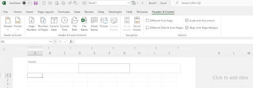
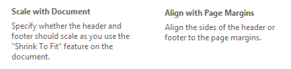
Notice the new ribbon tab, “Header & Footer” which gives you access to the items as icons we saw previously! Here are the definitions of the right-most checkboxes in the above illustration:

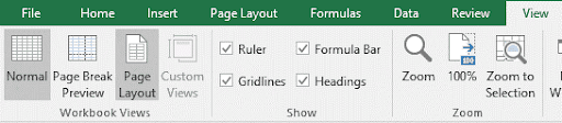
These different views of the spreadsheet are also visible from the ribbon’s View tab in the very left section, as seen here:

---