Standard Deviation & Variance in Python
Std Dev & Variance
Variance
Average squared distance from the mean. Units are squared (awkward to interpret).
Standard Deviation
Square root of variance. Same units as the data — easier to interpret.
Bell Curve Reference
~68% of data within ±1 SD of mean, ~95% within ±2 SD, ~99.7% within ±3 SD.
Python Code
import statistics; statistics.stdev(data) for sample SD, statistics.pstdev(data) for population.
Noble Desktop's Python Programming Immersive covers AI APIs, data analysis, and modern Python development.
Now that we discussed mean, median, and mode – let’s discuss a topic that is a bit more complex but is frequently used in finance, health, and many other sectors. The standard deviation or variance, the standard deviation is just the variance square rooted or raised to ½. The standard deviation is more commonly used, and it is a measure of the dispersion of the data. This is very different from the mean, median which gives us the “middle” of our data, also known as the average.
Sample Python Code for Standard Deviation
Standard Deviation Explained
Let’s go back to our example of test scores: 83,85,87,89,91,93,95,97,99,100. The average of these test scores is 91.9, while the standard deviation is roughly 5.5. So, what does this 5.5 really tell us about the test scores? The number 5.5 shows us how the numbers are spread out from the mean and 5.5 is a relatively low standard deviation score. This tells us that the data is fairly central to the mean and there are few if not no outliers in our dataset. If this is confusing for you, let’s take a look at the image below.
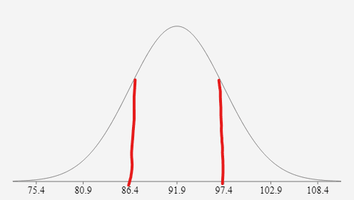
This image is a bell curve of our test scores data as you can see the middle of the curve is the value 91.9 which is our mean. Additionally, the red lines I drew on the curve show one standard deviation away from the mean in each direction. This means that I added 5.5 to 91.9 to get 97.4 and I subtracted 5.5 from 91.9 to get 86.4. One might not notice but 80.9 is the 91.9 – 2*5.5 and 102.9 is 91.9 + 2*5.5, and lastly, 75.4 is 91.9 – 3*5.5 and 108.4 is 91.9 + 3*5.5. Therefore, you might be thinking 108.4 or 75.4 was not in our dataset but that does not matter this is how you build a bell curve (by adding and subtracting to the mean by the standard deviation). There is no need to know why we do this (I promise there is a reason), but it is important to know how we got these numbers and how we use standard deviation in building a bell curve.
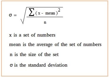
Now that we understand the definition of standard deviation and can visualize – how can we find it? Well before we know how to solve it, we must go over some Greek mathematical letters. Below is the full equation for standard deviation – if it seems very daunting do not worry, I will go over each variable and what it means. The lower-case sigma represents the standard deviation and the is equal to the square root of a complex fraction. The denominator of the fraction is encapsulated by an upper-case sigma which means it’s a continuous sum of the parenthesis. In the parenthesis, the X represents a specific data point in our set – mean and then we square it to get rid of any negative. We perform this on all the data points in the dataset and add up the result, once we get the final sum we divide it by the size of the dataset and take that number and square root it.
This is a complicated process and requires that the data stays the same since each data point is calculated individually and then added to an overall sum. Therefore, Python is great for a calculation of this sort as it does all the heavy manual calculations for us. It is important to note that writing a function for standard deviation using only Python code and no packages is virtually impossible for a beginner and intermediate programmers. Lucky us, the beauty of Python is the ease of importing packages to carry out various tasks. NumPy, Pandas, Matplotlib, and scikit-learn will all be discussed at length in later blog posts but for now, we will use the math package which comes with the basic Python build. This package is powerful but still does what Pandas can do in one step in a few different steps.
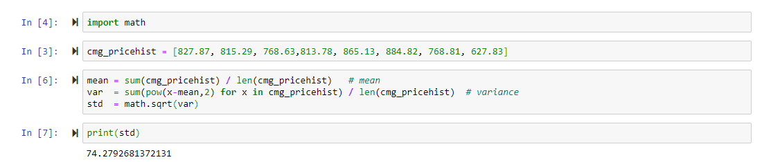
*In this code example I will be using financial data from a stock because standard deviation is a very commonly used metric when discussing volatility. The data is from the Chipotle’s stock, all of the pricing data in this example is real and is the ending price of the CMG at the first of each of the last eight months.
Step 1: Import math package
Step 2: Create a list called cmg_pricehist and set it equal to the eight closing values of Chiptole’s stock.
Step 3: Create a mean variable by taking the sum of cmg_pricehist and dividing it by the length of the list (the number of data points)
Step 4: Create a var variable and set it equal to a chain of commands: the first command is sum(pow(X-mean, 2) – this is the numerator of the standard deviation formula seen above, to cycle through each “X” we create a list comprehension here so that the sum and power function is applied to each data point.
Step 5: Create a standard deviation formula and set it equal to math.sqrt(var), this function takes the variance and raises it to ½.
Step 6: Print standard deviation variable
Now, ask yourself – would you consider Chipotle a volatile company or not?