Using Excel Tables

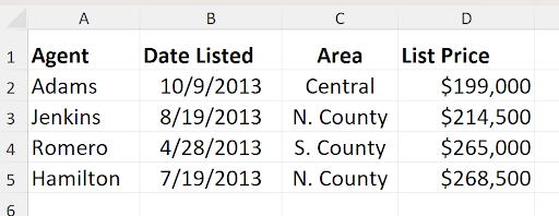
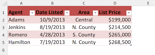
What is an Excel Table? Its structure is just a list of data, with no missing rows or columns. But when you tell Excel it’s a table, it takes on properties which are very useful to work with. For example, if you add data to the bottom, it’s automatically included in the table. Formulas automatically are filled down the column. References to the table take on a new syntax (which can optionally be turned off, and we’ll cover them later in this article).

Let’s look at data before and after it’s a table:

Before:

Then either of these methods:

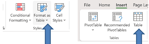
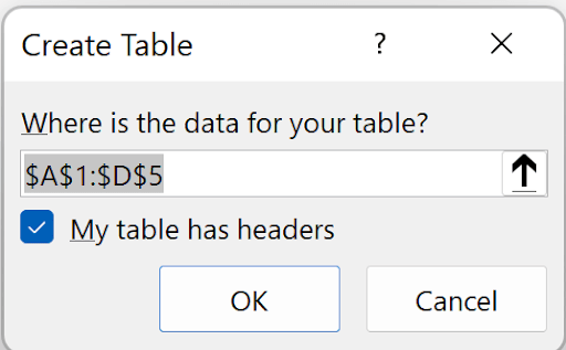
The illustration on the left is from the Home tab of the ribbon, and on the right is from the Insert tab. Either choice makes a table, but the one on the left first brings up a palette of color choices. They do the same thing, basically, and personally I think the label “Format as Table” is misleading, since it’s beyond formatting! Then:

After:

There’s a 3rd way to make a table, and that’s to press CTRL/T (or CTRL/L, a leftover from when it was referred to as a List).

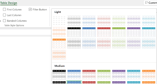
The color choice is flexible from the palette which is on the Table Design tab of the ribbon (which exists only when the active cell is inside the table). Here’s a part of the color choices (there’s more):

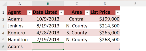
You can see from the first table shown that row 6 is empty, as is column E. If something is entered in A6, it’s obvious it was added to the table, because of the coloring:

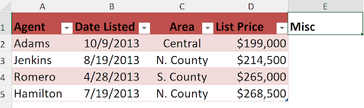
Or if something is entered in E1:

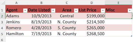
In both cases, you can leave the data you entered but not have it included in the table by pressing CTRL/Z (undo):

Okay, it’s a table. Now what? Let’s look at selecting a row or column. When you hover the mouse over column A, there are 2 different shapes possible.

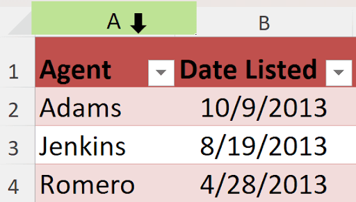
This is the usual shape before you click the mouse. If you do click here, you select all of column A. Then there’s this, if you move the cursor down just a little:

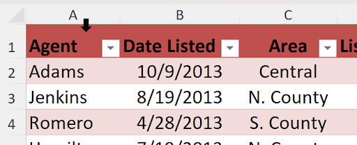
And if you click the mouse now, it selects only column A cells which are in the table, in this case, A2:A5. (A1 is not selected with this method). If you click here:

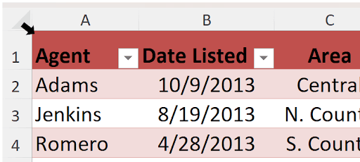
This cursor rotates and you can select the entire table (again, not the header row).

You can see the name of the table is shown as well:

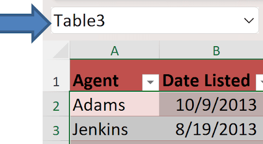
You can (and should) give your tables a more meaningful name!

If you start entering a formula referencing Table3, after the 3 you type a left square bracket, and you see this:

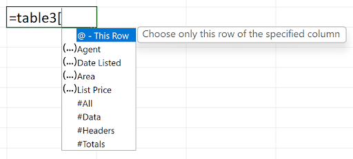
This is all new syntax, called structured referencing.

To refer to the row of the table in which the formula you’re entering is, you use the @-symbol:

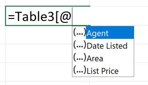
The dropdown displays a list of all the column headers in the table.

So, if you enter =Table3[@Area] in cell G4, say, then the data from the Area column will come from row 4. If you refer to a field which has special characters or a blank, another set of square brackets is used. For example, to refer to the Date Listed field, you’d use =Table3[@[Date Listed]].

#All is the entire table. #Data is the table without the headers. #Headers is the headers, and #Totals is the totals row. If there is no Totals row, this will return #REF!. How to put in a Totals row is shown below.

Once you create a table, you’re automatically presented with column filters.

Let’s take a look at the commands in the ribbon when the active cell is part of the table:

Properties

This is where you can give the table a meaningful name as well as resize the table – in this illustration, the table was from A1:D5, yet there’s data below, in rows 6 and 7 which are not part of the table (yet).

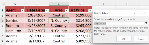
When you have the dialog shown, you can simply change the reference to be A1:D7:

Tools

• Some of these are pretty obvious and don’t really need a discussion, like Summarize with Pivot Table or Remove duplicates
• Convert to Range will remove the status as a table, but will keep the coloring.
• Insert Slicer (available for Tables and Pivot Tables, not regular ranges) will bring up the Slicer dialog (outside the scope of this article).

Export Table Data

• Outside the scope of this article

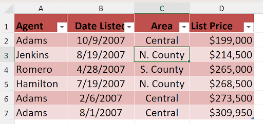
Table Style Options

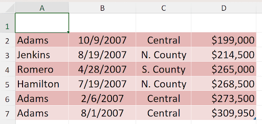
There are 7 checkboxes in this group. You can turn these on or off. By default, Header Row and Banded Rows are checked. I can’t imagine why you’d want to remove the Header Row, but you can. The table would look like this:

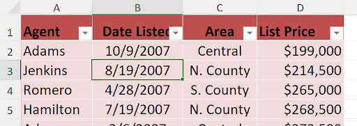
Banded rows gives the appearance of a slightly different shading to every other row. Without it:

Total Row will add a row to the table with the word Total and a total in the last column, using the SUBTOTAL(109, …) formula.

First Column is to give a shading to the first column:

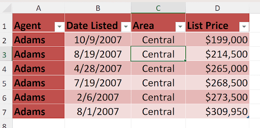
Similarly for the Last Column:

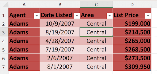
Banded Columns gives every other column a shade (here, the first, last, and Banded Rows were unchecked):

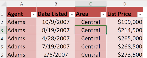
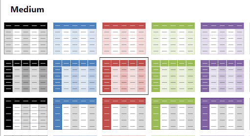
With each of the shading options, the gallery of styles is also updated. For example, with First Column and Banded Columns only checked (and Header Row), here’s a sample of the Medium styles in the gallery:

Filter button toggles the filters from the header row on or off.

Table Styles

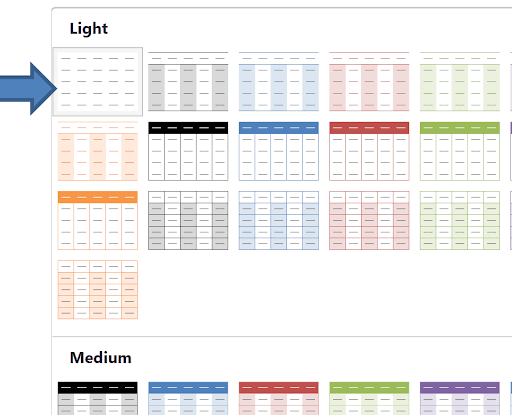
Obvious, but to make it not look like a table, you can select the top left icon:

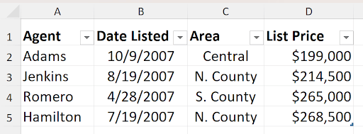
And the table looks like this:

By the way, if you don’t like the structured referencing, you can have Excel not apply it by a setting in File/Options – deselect “Use table names in formulas”: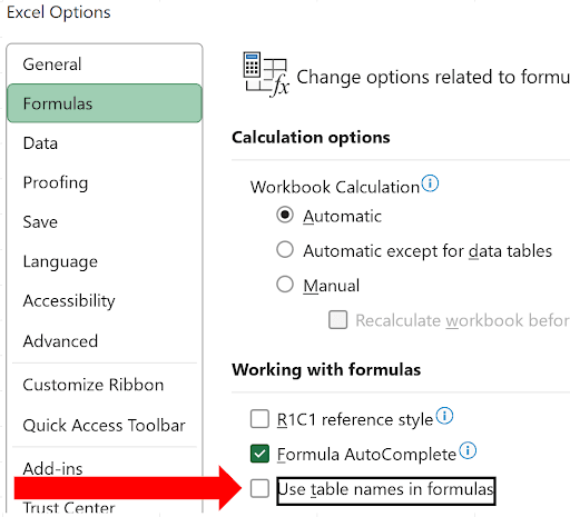

If a Pivot Table is based on a table (and it should be), as the table grows or shrinks, a refresh will refer to the correct data. If a Chart is based on a table, as the table grows or shrinks, the Chart is updated.