Filtering Data in Excel

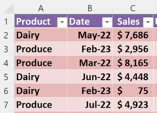
Filtering data means to show a list of data but only those rows which has information you’re interested in seeing. The other rows are hidden, or, more accurately, filtered. A simple example. Suppose you have this short list:

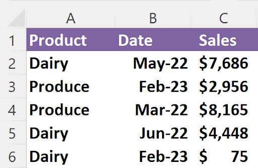
And you’re only interested in seeing the rows for Dairy. There are several ways to do this. First, let’s look at the result of that filtering:There are several things to notice:

The row numbers have turned blue

Rows 3-4 are not visible (they’re filtered)

There are icons in cells A1:C1

The icon in cell A1 has a filter icon, meaning this column contains the instructions for filtering that column’s data.

Let’s look at the many ways this can be done, then we’ll expand the scope of what filtering can do.

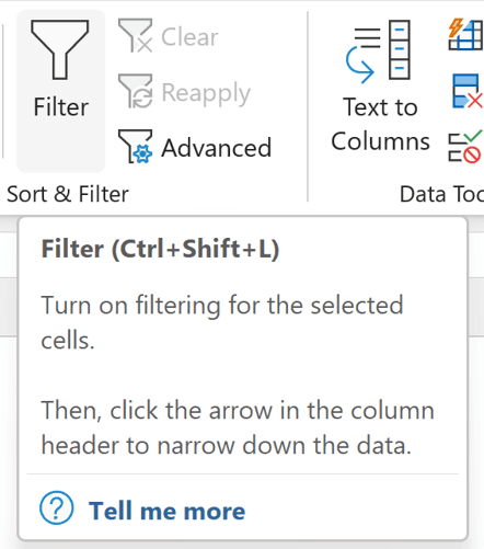
In the Data tab of the ribbon, the Sort & Filter group, you’ll see the Filter icon. You can click this or, as the tip says, press CTRL+Shift+L. This is a toggle to enter filter mode or exit it. The effect of soing this is that you’ll see the filter icons in every column, top row, of the region surrounding the active cell.

Right-click on the cell you want to filter by, and select Filter/Filter by Selected Cell’s Value:

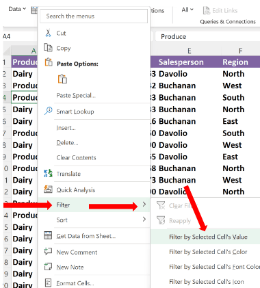
This will not only put you in filter mode, it will also do the filtering – in this case, filter by Produce.

When the filter icons are present, clicking on the arrow (Produce, in this example) will show this:

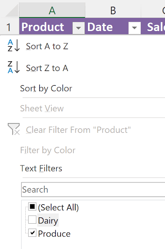
Notice there are several other features here, including Sorting in the top half. At the bottom is an option to select which item(s) you want to see. If there were many, then you can select (or deselect) the ones you want to see (or not want to see!)There’s also a Search box, in which you can enter something to search for. Here’s an example with a new dataset:

If I type Apple in the search box:

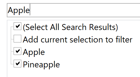
Notice Pineapple is also selected! There’s also a checkbox, “Add current selection to filter”. If I had previously filtered by Banana, for example, then clicked that checkbox above, I’d see:

---

There’s also a field called Text filters:

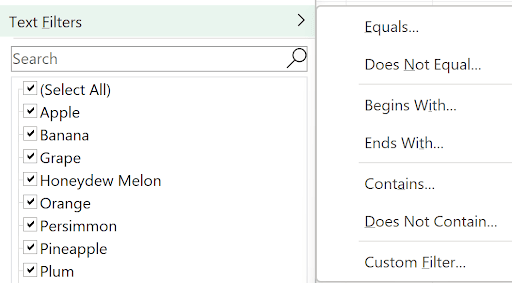
As you can see, there are many other features here. Instead of showing each one, since they’re fairly self-explanatory, I’ll show one, “Begins with…”:

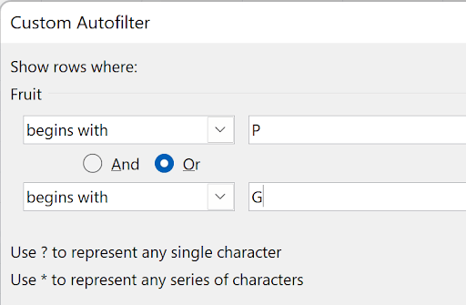
This choice would show:

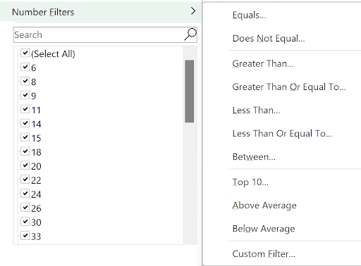
If the field is not text, you would see a different choice besides Text Filters:

1. Number filters

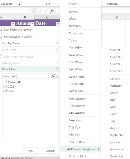
2. Date filters (Pretty massive choices here!)

Converting to a Table (covered in a separate article) will also put the filter icons at the top of each column and has many added features. It pretty much looks the same (going back to the original list) aside from applying some Table formatting:

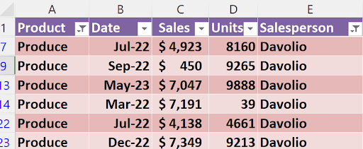
You can filter more than one field. Assume you have chosen just Product, you can then filter that choice by another column. For example, I can pick a particular salesperson:

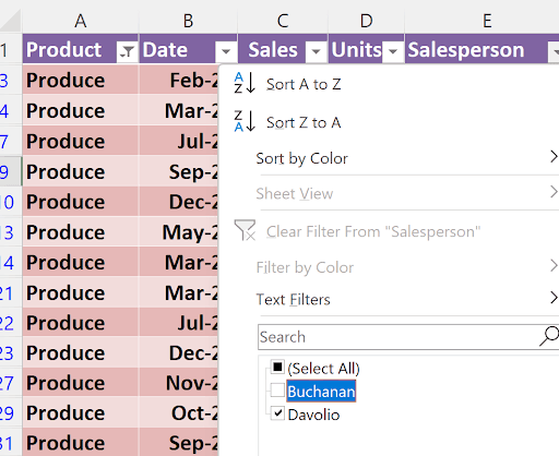
Which produces:

Then, further, I can pick items under,000 in sales:

---

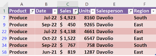
By the way, when you filter, you get a notification of the results at the bottom left of your screen:

The quickest way to show all records yet remain in filter mode is to press CTRL/Shift/L twice!

Near the beginning of this article, using the right-click and selecting Filter, there were several other options, repeated here:

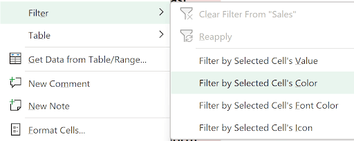
Without demoing each, here’s what they do:

Filter by Selected Cell’s Color is the color of the cell, not the font color. If your list is multi-colored, you can filter by a particular color!

Filter by Selected Cell’s Font Color is the font color of the cell, not the color.

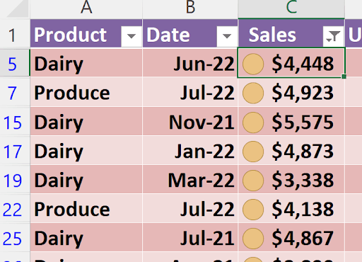
Filter by Selected Cell’s Icon is used if you chose icons from the conditional formatting feature:

This can show the data like this!

Then if I filter by right-clicking the $4,448, and select Filter by Selected Cell’s Icon, I’d see:

There’s much more to filtering. In another article we’ll cover Advanced Filtering, as well as review the new Dynamic Array function, =FILTER(…)