Collection of Excel Tips and Tricks, Part 1

This is the first of a series of articles on Excel tips and tricks. Let’s dive right in. In this workbook, there are 3 names defined:

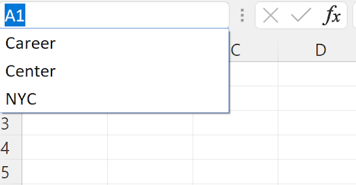
If I select NYC, I see this:

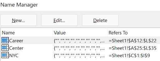
You can see in the name box (above column A) that NYC is the selected range. The other two ranges’ addresses can be seen here:

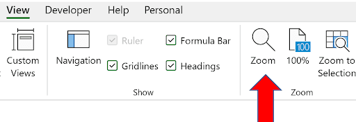
So what’s the tip/trick? Go to View/Zoom:

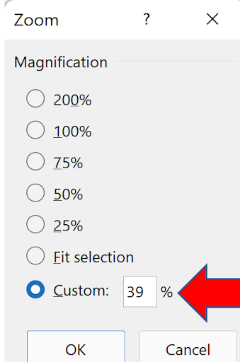
Select 39% (or less):

You will now see all range names show up (as long as they’re more than one cell wide or tall):

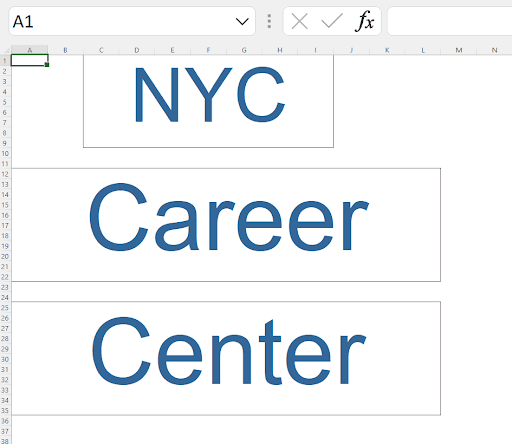
Pretty cool, eh?

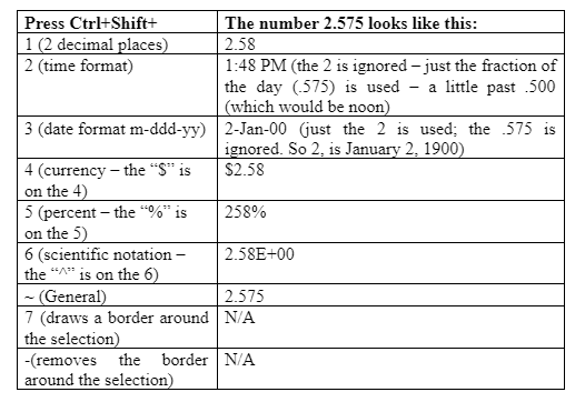
OK, let’s look at another set of tips. Here, we’ll examine many shortcut keys. They all involve holding CTRL+Shift down, then we’ll see the effect of using the values 1 through 6 and more: 

Here’s a tip on printing – suppose you have the page setup just the way you like it on sheet1, but you want to use the same setup on sheet2, or other sheets. Do you have to redo all the setup steps again? No – simply place the desired sheets to inherit the desired page setup into “group” mode. You do this by CTRL/clicking another sheet tab, or shift/clicking to put all the sheets between the active sheet and the one you shift/clicked into group mode. When you do this, you will see the word “Group” at the top:

---

Here's sheet1 preview:

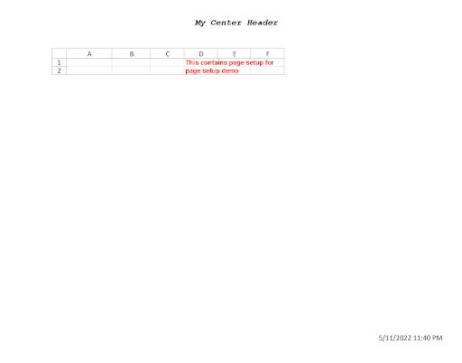
Note it’s landscape, has row and column headers showing, has a header of “My Center Header”, and date and time at the lower right corner.

Sheet2 has no settings. Once Sheet1 and Sheet2 are in group mode, and Sheet1 is the active sheet (the one with the settings you want to copy), you simply visit the Page Setup dialog and click OK:

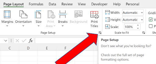
Then you see 🡪

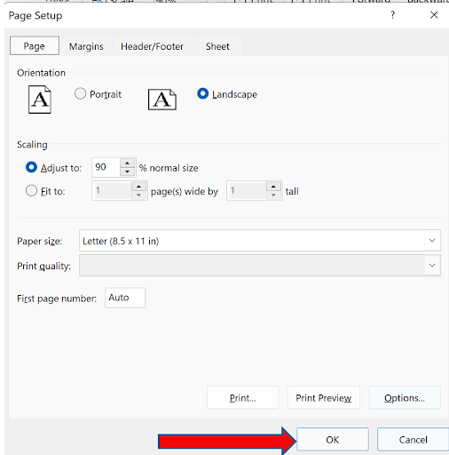
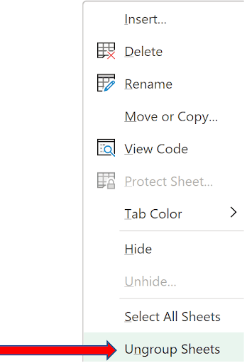
And that’s it. All the sheets in the group now have the same page setup as the active sheet. What’s left to do is take the sheets out of group mode. The easiest way to do that is to right-click the sheet tab and select Ungroup Sheets:

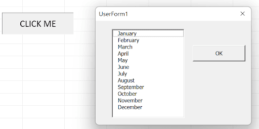
Here’s one for those of you who write VBA code and use Userforms. Here’s a simple userform that displays a listbox with the months in them:

How do you get the months in the list? I’d guess most either write initialize code to fill the listbox, something like this:

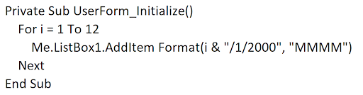
This works – the value of i the first time is 1, and formatting 1/1/,000 with MMMM is January. The day and year are pretty arbitrary.

Or something like this:

---

This also works, but is a lot of typing. Since the array is 0-based, the subscript is i-1 instead of i. We could have used i if the loop were For i=0 to 11. 

Another way would be to put the months in cells – pretty easy because you need only to type January then use the fill handle to get to December, like this:

And then in the user form design, you can select the listbox and simply point to that range in the Rowsource property:

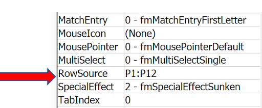
But here’s the tip – you don’t need any of those ways – there’s a direct way:

All you need in the initialize event of the form is one line:

What’s GetCustomListContents(4)?

In File/Options, the Advanced section, near the bottom is Edit Custom Lists:

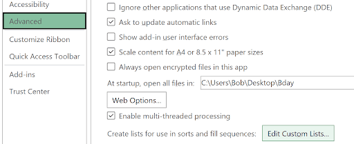
When you click this, you see:

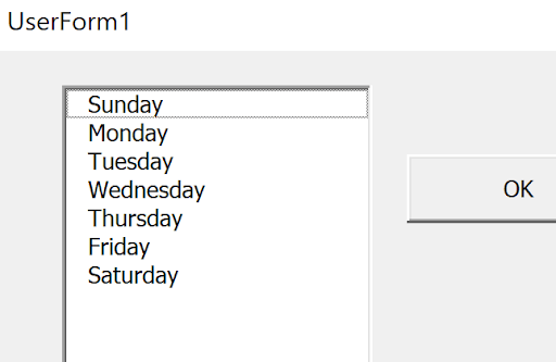
The 4th one of these is the list of months! You reference this list by Application. Getcustomlistcontents(4)! Had I tried Application. Getcustomlistcontents(2), I would have seen this:

Hope you enjoyed the first article of Excel tips & tricks.

---